One of the key behavioral relationships for households is the division of income between household consumption, C, and household savings (HHSAV). Given historic data, it is possible to estimate cross-sectionally a relationship between GDP per capita and average household consumption propensity.
It is, however, not possible to conceptualize and forecast household consumption independent of other expenditure components (government consumption, investment, and net trade). There are equilibrating mechanisms that cross over the goods and services market and influence agent behavior with respect to consumption, investment and savings.
The core of the consumption equation, calculating a preliminary estimate of household consumption (ConsumHHPrel), multiplies a consumption ratio (CRA) as a portion of disposable household income times that income. The consumption ratio floats over time, and it will be recomputed for the next time cycle at the end of the complete formulation for household consumption. That core is multiplied over time by a ratio of the expected household consumption as a percentage of GDP from the analytic function estimated above and the percentage that would have been expected given the GDP per capita in the previous time step.

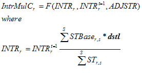
There are two additional factors in the above equation for household consumption, and the first is an interest rate multiplier (IntrMulC). Real interest rates (INTR) – IFs does not maintain a monetary sector that would introduce nominal interest rates – are a key equilibrating variable. IFs ties interest rates to the overall balance between production and consumption in the system as indicated by the sum across all sectors of desired stocks in comparison with actual stocks/inventories (ST). Desired stocks in IFs are determined by a stock base (STBase) linked to production and consumption levels and a desired stock level (dstl) as a portion of the stock base. Interest rates rise as stocks fall relative to desired levels and fall as stocks rise above those desired levels. Interest rates enter into the equation for total household consumption such that rising interest rates depress consumption.

Although it should perhaps be rolled into the interest rate formulation, IFs maintains a second variable for modification of the household consumption function, a multiplier on consumption (MulCon), that helps maintain the general equilibrium between domestic savings and GDP. (It is important to understand that total savings will identically equal investment, by calculation; but it is possible that foreign savings swings can dramatically influence savings totals in a fashion that would completely crowd out or greatly expand domestic savings were there no other forces working at equilibrating domestic savings.) As domestic savings rise as a portion of GDP, they cause the consumption multiplier to rise and therefore consumption to rise.

Having modified total household consumption, C, the preliminary household consumptions (ConsumHHPrel) of the different household types will no longer sum to it, so they are normalized to do so. The rates of consumption relative to disposable income can then re-computed.


It is also important to explain the initialization of those rates of consumption. In the first time step, those rates are calculated taking into account the differential propensity of different household types, currently limited to skilled and unskilled households, to consume and save. The differences are maintained over time.
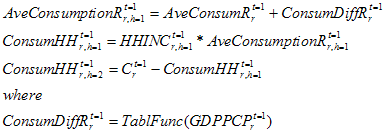
The average propensity to consume in the initial year (AveConsumR) can be calculated from data.

If both types of households consumed an equivalent share of income, they would consume at the average rate, as modified by the factors discussed above. Almost certainly, however, lower income, unskilled households have a higher average propensity to consume than do skilled households. In the absence of data-based knowledge about that, IFs currently uses a stylistic, and flexibly changeable function to represent the extent of that differential, assumed to decrease as GDP/capita increases.
The consumption differential from the function adjusts the average rate for unskilled households and allows computation of actual consumption (Consum) of the unskilled and a residual calculation of consumption for the skilled (subject to tests for positive sign and reasonable size, not shown below).
The differential propensity to consume is an important feature for scenario analysis, because transfers across household types are one of the key policy levers available to governments.


Savings terms are calculated as residuals for all agent classes, and are determined after all income and expenditure/transfer calculations. In the case of households they are income, minus consumption and net transfers to government.
![]()
IFs does not attempt to track assets and liabilities of households over time and to add that information to the behavioral representation of them. That might be useful in the future.