The core equation for the production function computes value added (VADD) from technology (TEFF), capital (KS), labor (LABS), and capacity utilization (CAPUT), with a time-constant scaling parameter (CDA) assuring that gross production is consistent with data the first year. GDP is, of course, the sum across sectors of valued added. Although the production function can serve all sectors of IFs, the parameters agon and enon act as switches; when their values are one, production in the agricultural and primary energy sectors, respectively, are determined in the larger, partial equilibrium models and the values then override this computation (see documentation on those models for detail).

where

Other topics in our documentation explain the dynamics underlying change in capital stock (through investment and depreciation) and labor supply (through demographic change and participation patterns). The rest of this topic will focus on the computation of the elements that go into the MFP or technology term (TEFF), working our way progressively deeper into their determinants.

At the most basic level the stock term is simply an accumulation of the annual increments in MFP. 

 where  1.0

The annual growth in MFP (MFPGRO) consists of a base rate linked to systemic technology advance and convergence (MFPRATE) plus four terms that affect MFP growth over time as a result of human, social, physical, and knowledge capital. 

Each of the following subsections elaborates one of the five terms.

Annual Base Technology Growth in MFP

The base rate related to technology or other factors unexplained by the four capital terms is anchored by an exogenous specification of the sector-specific rate of advance in the systemic leader’s technology ( mfpleadr ); the leader is assumed to be the United States. (The rate in the leader's ICT sector gradually convergences over time to that of the service sector.) On top of that is an endogenously computed premium computed for convergence of each country/region (MFPPrem), a term that is a function of GDP per capita at PPP, the function for which posits an inverted-V shape with the greatest potential for technological convergence to the leader among middle-income countries. In this calculation there needs to be a correction factor (MFPCor), computed to assure that the actual rate of this growth is consistent with the actual amount of growth for a country/region (MFPGRO) that is unexplained by capital and labor growth in the first model run year. That correction factor converges to 0 over the number of years specified by mfpconv . This convergence assumption has significant implications for model behavior because it tends to slow down growth in countries (like China) that have had a burst of growth beyond that which the rates of the leader and the catch-up factor would lead us to anticipate and to speed up growth in countries (like the transition states of Central Europe) that have suffered a reduction similarly unexpected by the basic formulation.

where

 and

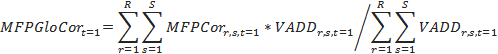
It is possible for the regionally and sectorally specific MFP correction terms (MFPCOR) to still leave a small discrepancy between the global economic growth in the data and the initial growth rate in the model. To avoid this, we also compute a global correction factor (MFPGloCor) as the region/country and value added weighted sum of the individual country-sector terms divided by the global and regional sums of value added.

In addition to the basic technology terms and the correction factors, there are three parameters in the MFPRATE equation (with zero values as the default) that allow the model user much control over assumptions of technological advance. The first is basic parameter ( mfpbasgr ) that allows a global growth increment or decrement; the second is a parameter ( mfpbasinc ) that allows either a constant rise or slowing of growth rate globally, year by year, where zy is the count of the model run years across time; finally is a frequently-used parameter ( mfpadd ) allowing flexible intervention for any country/region.

Driver Cluster 1: Human Capital

The general logic of each the four driver clusters around human, social, physical, and knowledge capital is the same. Each cluster aggregates several variables that generally contribute to productivity. For each variable, such as average years of adult education in the human capital cluster, there is an expected value and an actual value. It is the difference between actual and expected values that gives rise to a positive or negative contribution to productivity and growth. Most expected values are identified in a relationship with GDP per capita at PPP.

That is, there is a tendency for most developmentally supportive variables to advance in a rough relationship with each other and with GDP per capita (Kuznets 1959 and 1966; Chenery and Syrquin 1975; Syrquin and Chenery 1989; Sachs 2005). To the degree that they do, such advance can be understood to be consistent also with the overall technological advance of the country. If, however, a variables such as years of formal education attained by adults exceeds the typical or expected value for a country at a given level of GDP per capita, we can expect that variable to add something more to productivity. Similarly, falling behind the expected value could retard productivity advance. To illustrate and emphasize this point, even a country for which adult education levels advance could find that education is not keeping up with the advance in other developmental variables including GDP per capita and find that its education levels move from contributing to productivity enhancement to decrementing that productivity enhancement.

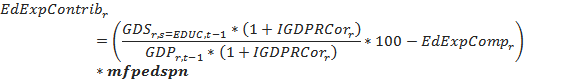
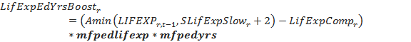
In the human capital cluster there are six variables that add to or subtract from the human capital (MFPHC) term: the educational spending contribution (EdExpContrib), the years of adult education contribution (EdYearsContribub), the boost from life expectancy years (LifExpEdYrsBoost) assumed to generate (via mfpedlifexp ) extra years of education, the stunting contribution (StuntContrib) related to undernutrition of children, the disability contribution (DisabContrib) related to morbidity from the health model, and vocational education contribution (edVoccontrib) resulting from growth (or decline) in vocational share of lower and upper secondary enrollment,. The first five of these six drivers have a similar formulation while the formulation for vocational education is slightly different. The first five, as computed in IFs often as a result of extended formulations and even other models of system (as with life expectancy, computed in the health model) are compared with an expected value. In the case of disability, the expected value is set to the world average level (WorldDisavg), but all other expected values (EdExpComp, EdYrsComp, LifExpComp, and StuntingComp) are computed as functions of GDP per capita at PPP. As the provision of vocational education does not follow any common pattern or trend and is rather a matter of policy choices made (or will be made) by the particular country, it was not possible to calculate an expected value for this variable We have instead computed the vocational education contribution from changes in vocational share over time with appropriate moving averages to capture the lag required in materializing such contribution and to smooth out the contribution over time. (Note: In the base case of the model, vocational shares do not change and as such EdVocContrib is zero).

In each case a parameter drawn from study of the literature and/or our own analysis converts the difference between actual and expected into a positive or negative contribution to MFP. (Because of the recursive structure of IFs, some terms rely on variables from the previous time step, estimated from the current time step with a correction factor based on initial GDP growth.)

where

where

Vocational contribution for lower secondary is calculated as:

A similar calculation is done for upper secondary vocational and the two are averaged as shown below:

Driver Cluster 2: Social Capital

The logic of comparison of actual with expected values is the same as that described above for human capital in the case of the six factors that contribute to social capital: economic freedom as in the Fraser Institute measure (EconFreeContrib), government effectiveness as in the World Bank measure (GovtEffContrib), corruption as in the Transparency International measure (CorruptContrib), democracy as in the Polity project measure (DemocPolicyContrib), freedom as in the Freedom House measure (FreedomContrib), and conflict as in the IFs project's own measure tied in turn to the work of the Political Instability Task Force (ConflictContrib). In each case other than that for conflict, the expected values (EconFreeComp, GovEffectComp, CorruptComp, DemocPolityComp, and FreeComp) are computed from functions with GDP per capita at PPP. In the case of conflict, the expected value is set at the initial year's value (and the comparison is reversed because lower conflict values contribute positively to MFP).

where

Driver Cluster 3: Physical Capital

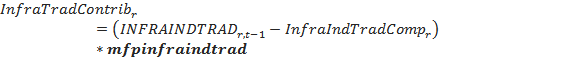
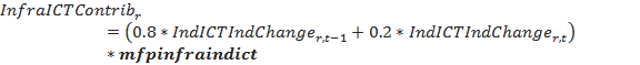
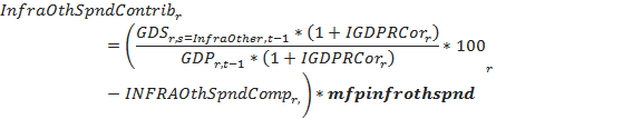
The logic of the physical capital cluster is again parallel to that of the human and social capital clusters and involves the comparison of an actual (that is, IFs computed) with an expected value. The formulation for MFPPC can actually take several forms depending on the value of a switching parameter ( inframfpsw ) but the standard form involves four contributions, from traditional infrastructure (InfraTradContrib), ICT infrastructure (InfraICTContrib), other infrastructure spending level (InfOthSpenContrib), and the price of energy (EnPriceTerm). The last term is included because higher prices of energy can make some forms of capital plant no longer efficient or productive.

In the case of this cluster only the expected value of the traditional infrastructure index (InfraIndTradComp) and the expected value of other infrastructure spending (InfraOthSpendComp) are computed as most other cluster elements are, namely as a function of GDP per capita at PPP. In the case of the ICT index contribution, the technology has been evolving so rapidly that there is not really a basis for an expected value with some stability over time. Instead the contribution from ICT is computed in terms of a moving average value of change over time, such that faster rates of change contribute more to MFP as the moving average expected value lags further behind the actual. In the case of the energy price term, the "expected" value is set equal to the energy price in the first year of the model run. As with other clusters and the variables in them, a single parameter links the discrepancy between actual and expected values to MFP.

where

where

Driver Cluster 4: Knowledge Capital

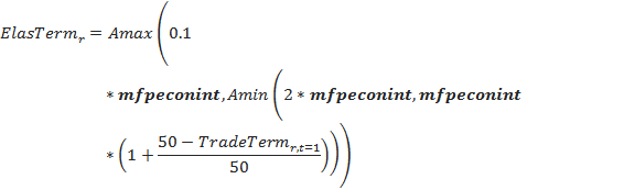
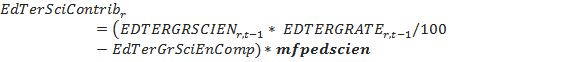
Following the pattern of other MFP driver clusters, the one for knowledge accumulation includes terms that compare actual model and typical or expected values and use parameters to translate the differences into increments or decrements of MFP. In this case the three terms represent R&D spending (RDExpContrib), economic integration via trade with the rest of the world (EIntContrib) and the share of science and engineering among all tertiary degrees earned (EdTerSciContrib). In the first and third case the expected value (RDExpComp; EdTerGRSciEnComp) is a function of GDP per capita at PPP. In the second instance, there is no clear relationship between extent of economic integration and GDP per capita, so the model compares a moving average of trade openness (exports plus imports as a percentage of GDP) with the initial value of openness (because trade is computed later in the computational sequence for each year, the values of trade variables lag one year behind those of the production function). Given the extreme global range of trade openness, the elasticity term itself in this relationship is variable, with values decreasing when initial openness is greater (that is, countries that start with less openness gain more from the same percentage point increases in it).

where

where

Issues Concerning Parameterization and Interaction Effects

Although our approach to calculation of MFP creatively connects developments in many other models in the IFs system to it, parameterization of the effects individually and in interaction is complicated and uncertain. Hughes (2005) documented the original creation of the structure and its parameterization based on existing literature.

One of the concerns with this approach is the possibility of double counting of effects from the large number of variables fed into the MFP calculations. In general the project has dealt in part with this by selecting conservative values for the parameters when studies indicate possible ranges of contribution of the variables to productivity and/or growth. Another concern is that a very large or extreme advance by one or a small subset of variables could have inappropriately large impacts of productivity given the fundamental conceptual foundation of the approach in the notion that development involves widespread and reinforcing structural changes across many variables. In order to limit this possibility, we have created an algorithmic function (MFPContribAdj) to adjust the multiple MFP contributions and dampen especially high positive or negative contributions of the four cluster terms (MFPHC, MFPSC, MFPPC, and MFPKN). 

The Relationship of Physical Models to the Economic Model

IFs normally does not use the economic model's equations representing MFP and production for the first two economic sectors, because the agriculture and energy models provide gross production for them (unless those sectors are disconnected from economics using the agon and/or enon parameters). Instead, the two physical models provide gross production, translated to value terms, back to the economic model. See Section 3.2.3 for discussion of gross production.

In addition to this impact of the physical models on the economic model, there is one more of importance. Physical shortages on energy may constrain actual value added in each sector (VADD) relative to potential production. Economists typically do not accept such shortages as a real world phenomenon because (at least in theory) prices rise to clear markets; yet periods like the 1970s when governments intervened in those markets, such shortages do appear and they can in some IFs scenarios. In those situations, IFs assumes that energy shortages (ENSHO), as a portion of domestic energy demand (ENDEM) and export commitments (ENX) lower actual production in all sectors through a physical shortage multiplier factor (SHOMF). A parameter/switch ( squeeze ) controls this linkage and can turn it off.

where

In addition, the translation of potential into actual production depends on the imports of manufactured goods (MKAV), which serve as a proxy for both availability of intermediate goods and for technological imports. A parameter (PRODME) also controls this relationship.

Although the IFs model represents prices in real terms (no monetary sector and no inflation), there are relative sectoral price changes (PRI). Some of those can be quite dramatic over time, especially in the agricultural and energy sectors where the equilibration of physical representations of supply and demand can swing those prices. Such relative price swings can, in the real world, give added drag or boost to the value added in certain sectors and for economies as a whole. To represent this we compute a relative-price adjusted version of value added (VADDRPA), which is the normal value added weighted by world sectoral prices (WP); the prices are lagged a year because of the recursive model structure.