Forecasting of variables that relate to broader regime capacity in IFs has three elements: (1) a basic statistical formulation; (2) a recognition of country-specific differences (tied in part to path dependencies); (3) an algorithmic linkage to internal conflict. A fourth potential element could be factors external to the country including global waves and neighborhood effects, but we introduce those only through scenario analysis.

Corruption is one of the most powerful indicators of capacity (or more accurately, lack of capacity) as well as accountability. We rely in our analysis on the Transparency International index of corruption perceptions (CPI), which is actually a measure of transparency (higher values are more transparent or less corrupt). The basic formulation in IFs for corruption/transparency (below) contains four statistically significant drivers, which collectively account for nearly 80 percent of the cross-country variation in corruption in the most recent year of data. The first term, and the one identified with the most variation, involves a variable representing long-term development, namely GDP per capita (years of education plays that same role in forecasting formulations for some other governance variables, such as democracy).

Interestingly, a second very powerful driving variable is the Gender Empowerment Measure (GEM), which, in spite of its high correlation with GDP per capita, makes its own contribution and suggests the power of inclusion in affecting capacity. In fact, still another driving variable is the extent of democracy, further suggesting the power that inclusion may have to increase accountability and transparency, reducing corruption. A less-powerful but still-significant variable is the dependence of the country on exports of energy—in a few years, and in the aftermath of the Arab Spring beginning in 2011, this term may drop out of cross-sectional analyses of change in governance capacity but will still probably remain very important for those countries with low levels of development and inclusion. (We find that the same drivers work well (an R-squared of 0.62) for the IFs economic freedom variable, based on the Fraser Institute/Economic Freedom Network measure.) A multiplier for scenario analysis is the only exogenous element added to the basic formulation.

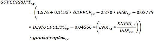
where

GOVCORRUPT= the Transparency International corruption perception index (for which higher values are more transparent or less corrupt)

GDPPCP=GDP per capita at purchasing power parity in thousand dollars

GEM=Gender Empowerment Measure (values below 1 indicate female disadvantage)

DEMOCPOLITY=Polity’s 20-point scale of democracy; inverse relationship

ENX=energy exports in physical terms (billion barrels of oil equivalent)

ENPRI=energy price per barrel

GDP=gross domestic product in billion constant 2000 dollars (market prices)

govcorruptm=an exogenous multiplier for scenario analysis

R-squared in 2010 = 0.75

We compute an additive adjustment term (not shown in the equation) on top of the basic formulation in the base year to capture any difference between the value anticipated in the formulation and the value from data. In most of our formulations we use additive or multiplicative terms in this manner, and the adjustment term introduces the impact of other variables not in the statistically estimated equation (such as historical path dependencies and cultural differences). The additive adjustment term gradually converges to zero over time in our forecasts. The logic behind such convergence is twofold: first, many differences from initial anticipated values are the result of transient factors and even data errors; second, ongoing global processes tend to lead to a convergence of patterns across countries.

There is every reason to believe that the presence of domestic conflict will reduce governmental capacity, including leading to lower levels of transparency (higher corruption). In fact, the inverse relationship between the IFs internal war variable (SFINTLWARALL) and transparency is strong. Even when added to the full equation above it remains quite strong (a T-score of -1.97). Because conflict tends to be quite variable over time, however, we undertook more analysis rather than simply adding conflict to the equation for corruption. Specifically, we experimented with different coefficients in analysis across the historical period (1960-2010). In doing so, we reinforced the result of the pure statistical analysis that a movement from 0 (no conflict) to 1 (conflict) appears to increase corruption (to lower the TI measure) by 0.6 points. We algorithmically overlaid this relationship on the basic equation above.

There are times when the user will wish to introduce normatively controlled target values for corruption. One approach is use of the "brute force" multiplier on corruption ( govcorruptm ). A second approach involves the specification of target values relative to a function of the key drivers estimated cross-sectionally across countries. This second approach allows, for instance, the specification of a target level 1 or 2 standard errors (SE) above the level expected of a country given those drivers. The SE target parameter is govcorruptsetar and the govcorruptseyrtar carries the years to achieve the target. Relevant to the discussion below, there are similar control parameters for regulatory quality ( govregqualsetar and govreqqualseyrtar ) and for effectiveness ( goveffectsetar and goveffectseyrtar ), but not for economic freedom.

Looking beyond the corruption/transparency measure of Transparency International, IFs also forecasts a number of capacity-related variables from the World Bank's World Governance Indicators project (Kaufmann, Kraay, and Mastruzzi 2010) that we did not use to define the capacity dimension, but that are still of significant interest (used, for instance, in forward linkages to the building of infrastructure). These include the quality of government regulation and government effectiveness. The approaches are identical to those used for corruption and involve the same drivers. The R-squared values are again high (0.74 and 0.72, respectively).

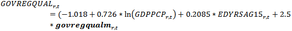
where

GOVREGQUAL=government regulatory quality using the World Bank WGI scale, shifting it 2.5 points so that it runs from 0-5 instead of from -2.5 to 2.5

GDPPCP=GDP per capita at purchasing power parity

EDYRSAG15=average years of education for adults aged 15 or older

govregqualm=an exogenous multiplier for the model user

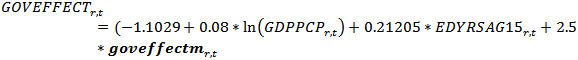
where

GOVEFFECT=government effectiveness using the World Bank WGI scale, shifting it 2.5 points so that it runs from 0-5 instead of from -2.5 to 2.5

GDPPCP=GDP per capita at purchasing power parity

EDYRSAG15=average years of education for adults aged 15 or older

goveffectm=an exogenous multiplier for the model user

We have also computed multivariate functions (using GDP per capita and education as drivers) for the other four WGI measures, voice and accountability, political stability, corruption, and rule of law. But we have not yet added them to IFs.

Turning to policy orientations, we compute an economic freedom variable based on the measures of the Economic Freedom Institute (with leadership from the Fraser Institute; see Gwartney and Lawson with Samida, 2000):

where

ECONFREE= economic freedom using the Fraser Institute/Economic Freedom Network freedom indicator (higher values are freer)

GDPPCP=GDP per capita at purchasing power parity

econfreem=an exogenous multiplier for the model user

R-squared = .5038