The energy model in IFs keeps track of trade in energy in physical quantities; the trade in energy in monetary terms is handled in the economic model.  As opposed to the agricultural model, where trade in crops, meat, and fish are treated separately, the energy model considers trade in energy in the aggregate.  Furthermore, it only considers production from oil, gas, coal, and hydro as being available for export.  Finally, as with other aspects of trade, IFs uses a pooled trade model rather than representing bilateral trade.

The first estimate of energy imports and exports by country are determined based upon a country’s propensity to export, propensity to import, and moving averages of its energy production and demand.

The moving average of energy production, identified as smoothentot, is calculated simply as a moving average of production of energy from oil, gas, coal, and hydro. In the first year of the model:

where

• e is oil, gas, coal, and hydro

In future years,

where

• e is oil, gas, coal, and hydro

The moving average of energy demand, identified as smoothpendem has a few more nuances, particularly after the first year.  In the first year, IFs calculates:

In future years, rather than using the value of ENDEM calculated earlier, the model uses a slightly different measure of energy demand, referred to as pendem.  pendem differs from ENDEM in two main ways:

1. rather than using the moving average country-level price index, renpri, to calculate the effect of prices on energy demand, it uses only current values:

^[1]

2. it does not include the additional boost in energy efficiency beyond enrgdpr in calculating the autonomous changes in energy efficiency

Thus, in future years, we have

A country’s propensities to import and export energy are given by the variables MKAVE and XKAVE.  These are moving averages of the ratios of imports to an import base related to energy demand and exports to an export base related to energy production and demand, respectively.  MKAVE is initialized to the ratio of energy imports to energy demand in the first year.  A maximum value, MKAVMax is also set at this time to the maximum of 1.5 times this initial value or the value of the parameter trademax .  XKAVE is initialized to the ratio of energy exports to the sum of energy production from oil, gas, coal and hydro and energy demand from all energy types in the first year.  Its maximum value, XKAVMAX is set to the maximum of this initial value and the parameter trademax .  The updating of MKAVE and XKAVE occur after the calculation of imports and exports, so we will return to that at the end of this section.

The initial estimates of energy exports, ENX, and energy imports, ENM, are calculated as:

where

At this point, IFs makes some adjustments to energy imports and exports depending upon whether a country is considered in energy surplus or deficit.  Where a country sits in this regard involves considering domestic and global stocks in addition to current production and demand.

Domestic energy stocks are computed as the sum of stocks carried over from the previous year, while also considering any shortages

A stock base is also calculated as 

The ratio of stocks to StBase can be defined as domesticstockratio. A moving average of a trade base, smoothtradebase, is also calculated for each country:

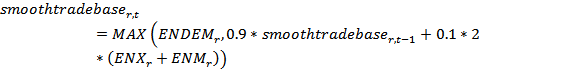
where

Global energy stocks, GlobalStocks, and the global stock base, GlobalStBase, are the sum of the domestic stocks and stock bases across countries, and the value of the globalstockratio is defined as GlobalStocks divided by GlobalStBase.

For each country, the level of deficit or surplus, endefsurp, is calculated as:

This implies that if a countries stock ratio is less (greater) than the global average, it is considered in deficit (surplus).

If a country is in deficit, i.e., endefsurp > 0, IFs will act to reduce its exports and increase its exports.  The recomputed value of exports is:

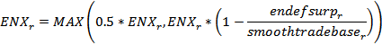
In words, the decrease in energy exports is determined by the ratio of the level of deficit to the smoothed trade base, but can be no greater than 50 percent.

The recomputed value of imports is:

with a maximum level given as:

Similarly, if a country is in surplus, i.e., endefsurp < 0, IFs will act to increase exports and reduce imports.  The amount of increase in exports is controlled, in part, by the exchange rate for the country, EXRATE, specifically its difference from a target level of 1 and its change from the previous year.  As with other adjustment factors of this type, the ADJSTR function is used, yielding a factor named mul.  After first multiplying ENX by a value that is bound from above by 1.05 and from below by the maximum of 0.95 and mul, the recomputed value of ENX is:

Here, a maximum level is given as:

where this maximum value is computed prior to the adjustments to ENX noted above.

The recomputed value of imports is:

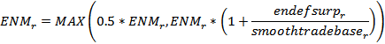
In words, the decrease in energy imports is determined by the ratio of the level of surplus to the smoothed trade base, but can be no greater than 50 percent.

Because of the frequent use and importance of government trade restrictions in energy trade, model users may want to establish absolute export ( enxl )  or import ( enml ) limits, which can further constrain energy exports and imports.  An export constraint may also affect the production of oil and gas as described in the next section.

As it is unlikely that the sums of these values of ENX and ENM across countries will be equal, which is necessary for trade to balance.  To address this, IFs computes actual world energy trade (WET) as the average of the global sums of exports and imports.

and recomputes energy exports and imports, as:

This maintains each country’s share of total global energy exports and imports.

IFs can now update the moving average export (XKAVE) and import (MKAVE) propensities for the next time step.  This requires historic weights for exports ( xhw ) and imports ( mhw ), yielding the equations:

A further adjustment is made related to the import propensity, MKAVE, related to the difference between this propensity and a target level, ImportTarget, and the change in this difference since the previous year.  This target starts at the level of MKAVE in the first year and gradually declines to 0 over a 150 year period.  As in many other situations in IFs, this process makes use of the ADJUSTR function to determine the adjustment factor.  The value of mulmlev is not allowed to exceed 1, so its effect can only be to reduce the value of MKAVE.

Finally, XKAVE and MKAVE are checked to make sure that they do not exceed their maximum values, XKAVMAX and MKAVMAX, respectively.