One of the key behavioral relationships for households (and a very important one for the larger model) is the division of income between household consumption, C, and household savings (HHSAV). Many factors affect that division including (1) an inertial element of consumption in the face of changing household income, (2) the relationship between GDP per capita and the propensity of households to consume from income (it tends to drop slowly), (3) the age structure of the population (people tend to consume a smaller proportion of income in the mid working years of life), (4) interest rates (high rates divert some income to savings), (5) life expectancy (longer life expectancy beyond retirement age should lead increase savings propensity). This section will address each of these in turn.

It is, however, not fully possible to conceptualize household consumption independent of other expenditure components (government consumption, investment, and net trade). There are equilibrating mechanisms that cross over the goods and services market and influence agent behavior with respect to consumption, investment and savings. Other topics cover those interacting representations.

The permanent income foundation of consumption

Households have ongoing consumption needs and patterns. Thus their consumption tends not swing as widely as does income. For that reason we begin by computing an internal model variable defined in the literature (e.g. Pistaferri 2001) as permanent household income (HHDisIncPerm). The computation uses a weighted average to smooth changes of permanent income in the face of changes in actual annual disposable income (HHDispInc).

The sum permanent income across household types yields total household permanent income (TotHHIncPerm).

Basic consumption computation and the affect of GDP per capita

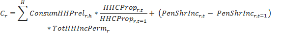
The core of the consumption equation involves calculating a preliminary estimate of household consumption for each of the two household types (ConsumHHPrel) by multiplying a consumption ratio (CRA) as a portion of permanent disposable household income times that income. The consumption ratio is carried along from year-to-year, providing an additional inertial but moving element of consumption (we will update it after finalizing the computation of consumption).

Our own cross-sectional analysis confirms a tendency for the consumption share of income to decline somewhat with increases in GDP per capita. We use that function to calculate the average household consumption propensity (HHCProp). The second term in the computation of consumption (C) adjusts the preliminary computation by household with the change of this propensity over time.  The third term adjusts this consumption term based on change over time in the ratio (PenShrInc) of government to household pension transfers (GOVHHPENT) to the total permanent income, assuming that pensions are mostly consumed.

where

Many countries have initial consumption shares of GDP that are especially high or low for a variety of historical reasons (high receipt of external assistance or remittances can boost C and governmentally-induced savings can reduce it). So we also set up a very slow convergence of C toward the more typical cross-sectional pattern for it, using again the household propensity to consume to drive C toward that target value (CTarget) in one of our standard IFs functions, ConvergeOverTime. The target is a portion of the potential, relative price adjusted GDP (GDPPOTRPA), again adjusted by changes in pensions.

where

The impact of age structure on consumption

Modigliani (1976) sketched the pattern of life-cycle savings and consumption and many others have followed (e.g. Lee and Miller 1992, Zhang and Zhang 2005, Zhang and Zhang 2009, Lee and Mason 2011). Consumption as a portion of income tends to be lowest during the peak working years and higher for the young and the old and/or retired.

Drawing especially on Lee and Mason (2011) we structured a relationship between marginal propensity to consume and age (the percentage portion of additional household income that would typically be consumed at different ages). We use that to differentiate consumption demands or needs of the population prior to working years (CPREWORK), during working years (CWORKING) and in retirement (CRETIRE). The function is used to compute an estimate of the percentage of additional income that each of the three groups consumes (YouthCon, WorkerCon, and PensionCon).

At this point there is a potential diversion from the normal flow of computation is the parameter cpctnduse (C percent response to balance between the savings need and expected availability for use) has been assigned a value larger than its normal 0.0. If the value is positive, SavingsNew and SavingsOld terms are calculated using an annuity formula (PV = C * [(1-(1+i)^-n)/i]) that is meant to assure adequate retirement income when C is set to 20.

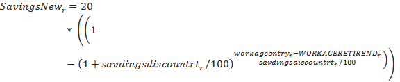
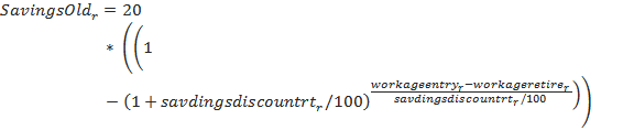
The difference between the new and old savings suggests the additional (or lesser) savings needed.

A portion of that (determined by the same optional parameter) can be subtracted from the consumption of workers so that they will instead save more.

Returning to the flow of computations regardless of the value of cpttnduse , we also compute the share of the three groups in the total population.

That allows an estimate of the share that each group would have of the total household consumption.

The sum of the consumption shares follows.

The difference between that sum of shares and its initial value provides basic information on how the changing age structure of a population across the three groupings will typically affect consumption intensity. Multiplying that by the permanent disposable household income (HHDisIncPerm) suggests whether consumption might likely rise or fall relative to our more inertial estimate of it, and by how much. The Aging Adjustment (normally populations are becoming older, but not necessarily so the term could be negative) is added to our earlier and more basic calculation of consumption.

This revised consumption can then be divided among the population-age categories.

A normalization process assures that the three terms sum to C.

The impact of life expectancy on consumption

The logic around changing consumption in response to age structure does not take into account life expectancy. To do that a life expectancy term (LifExpTerm) further adjusts consumption (and also gross capital formation, IGCF). That term responds to a life expectancy gap (LifExpGap) compared to the value of the gap in the first year; the gap itself compares actual life expectancy (LifExp) with a value for expected value based on GDP per capita at PPP (GDPPCP). 

where

Interest rates, stocks (inventories) and consumption

The trade-off for households between consumption and savings also responds to prices, both those of financing (interest rates) and those of goods and services. In IFs, both of those prices in turn respond to levels of inventories in the production/consumption sectors (called stocks (ST) inside IFs).

The modeling of the influence of interest rates could be done with the primary target being household savings. We instead represent the impact of rates on consumption, making savings the residual. The impact of interest rates on consumption is via an interest rate multiplier term (IntrMulTermC) that rise or falls over time as a function of the difference between a smoothed interest rate term (SmoothIntr) and a very long-term or highly-smoothed interest rate term (LongTermIntr). That is, as the smoothed interest rate rises above the long-term interest rate, it depresses consumption (and will therefore raise savings). In IFs there is no monetary sector and interest rates are real rates, not nominal ones.

Although we could similarly use the real prices of goods and services to affect consumption, the recursive structure of the model means that prices are computed in the supply/demand balance and not available at the time of this adjustment to consumption (the same lag issue affects interest rates, but the lagged values change slowly and using them is not a problem). To bypass the lag, the implicit price effect on consumption is introduced directly via an additive term reflecting half of excess stocks; the reason for passing through an adjustment of that magnitude is that household consumption is generally well above have of the total economy. Excess stocks are the difference between actual and desired stocks, which are determined by a stock base (STBase) linked to production and consumption levels and a desired stock level (dstl) as a portion of the stock base.

where

Savings rates and consumption

Were IFs to make savings rates responsive to interest rates and prices, rather than making consumption responsive to them, the formulation would most likely identify some long-term target value of savings rates and allow the actual value to rise above or fall below that based on driving values such as interest rates. Since IFs works primarily on consumption and makes savings the residual, it would be possible that savings rates are pushed unreasonably high or low. Moreover, it is possible that foreign savings swings can dramatically influence savings totals in a fashion that would completely crowd out or greatly expand domestic savings were there no other forces working at equilibrating domestic savings.)

To avoid this we make an additional adjustment to consumption using a multiplier on it (MulCon) that is responsive to the level of household and firm savings (HHSAV and FIRMSAV) as a portion of relative price adjusted potential GDP (GDPPOTRPA). That current household and firm savings rate (HHFirmSavR) is compared with a targeted one (HHFirmSavTarget) and the multiplier is computed in our standard IFs PID adjuster function (Adjstr). The target rate also uses one of our standard IFs functions, namely ConvergeOverTime, which causes it to gradually move from the initial rate to 30 percent over 80 years.

where

Investment and consumption

The introduction of a scenario to change investment/gross capital formation (IGCF) can be done in IFs using the multiplicative parameter on investment ( invm ). That parameter varies around its base value of 1. Rapid scenario changes can complicate model adjustment. Therefore, an adjustment term (IAdj) is calculated based on the difference between the parameter and 1.0, and that adjustment factor is subtracted from consumption.

where

Of course, the same amount needs to be added to investment.

Consumption by household type and update of consumption propensity for future years

Having modified total household consumption (C) the preliminary household consumptions (ConsumHHPrel) of the different household types will no longer sum to it, so they are normalized to do so. 

The rates of consumption relative to disposable income (CRA) can then be re-computed and saved for the next year for use in the preliminary calculations of consumption prior to the various adjustments of C.

The split of household consumption between unskilled and skilled households is maintained as a constant in this process. That is not ideal, but we have developed no alternative formulation at this point. But is therefore also important to explain the initialization of those rates of consumption by household type. In the first time step, those rates are calculated taking into account the differential propensity of populations at different levels of income to consume and save.

The average propensity to consume in the initial year (AveConsumR) can be calculated from data.

If both types of households consumed an equivalent share of income, they would consume at the average rate. Almost certainly, however, lower income, unskilled households have a higher average propensity to consume than do skilled households. In the absence of data-based knowledge about that, IFs currently uses a stylistic, and flexibly changeable function to represent the differential consumption propensity at different income levels, assumed to decrease as income (proxied by GDP/capita at PPP) increases.

The consumption differential from the function adjusts the average rate for unskilled households and allows computation of actual consumption (ConsumHH) of the unskilled and a residual calculation of consumption for the skilled (subject to tests for positive sign and reasonable size, not shown below).

The differential propensity to consume is an important feature for scenario analysis, because transfers across household types (and resultant changes in relative disposable income) are one of the key policy levers available to governments.

where

This allows then that initial year estimate of consumption propensity that will vary by household type with that variation carrying over across time, even as the rate of consumption for each household type rise and fall together as the consumption share of household income rises and falls.

Household savings

Savings terms are calculated as residuals for all agent classes, and are determined after all income and expenditure/transfer calculations. In the case of households they are income, minus consumption and net transfers to government.

IFs has begun to track assets of households in total over time as an element of looking at retirement financing, but not yet begun to do that by household type so as to add that information to the behavioral representation of household-specific savings. That might be useful in the future.