In years beyond the base year the total of government expenditures is calculated from the sum of direct consumption and transfers. The two components, however, each require a moderately complex calculation. There are no dynamics yet in place within IFs for local government expenditures (GOVEXPLOCAL).

Government Consumption

Computation of government consumption (direct expenditures on the military, education, health, R&D, foreign aid, and other categories) begins with use of a function to compute estimated government consumption (EstGovtConsum) as a portion of GDP, using GDP per capita (PPP) as the driver. The function supports a behavioral assumption of generally increasing expenditures with increases in GDP per capita (although the rate of increase is very slow).

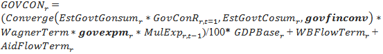
The estimated value then enters a convergence calculation that IFs uses in a number of instances. In the first year a ratio term (GovConR) was computed that represented the degree to which a country’s consumption/GDP differed from the estimated value. That ratio multiplies the estimated term in future years, allowing the function normally to increase consumption/GDP as GDP per capita rises. At the same time, such divergence from estimated functions is almost as often a matter of data inadequacy or of temporary factors for a country as it is of persistent idiosyncrasy. The convergence function allows the country/region’s value to converge towards the functional calculation over a period of time ( govfinconv ), usually quite long. Such convergence also helps avoid ceiling effects (e.g. government consumption as 100% of GDP) as GDP per capita rises.

The second term in the equation below is called the Wagner term, after the discoverer of the long-term behavioral tendency for government consumption to rise as a share of GDP, even at stabile levels of GDP per capita. This is built into the consumption calculation through an exogenous parameter ( wagnerc ) that is multiplied by the number of the forecast year (at the time of this writing the coefficient’s value was 0). The result of the convergence process and the multiplicative terms is divided by 100 and multiplied by a GDPBase term. The GDP base term could just be GDP. But relative price adjustments in countries can greatly affect government consumption—for instance, rising and falling relative oil prices can sharply affect government revenues and expenditures in oil-rich countries like those of the Gulf. Hence we arbitrarily add half of the difference between the GDP relative price adjusted value (GDPRPA) and the GDP to the base from which we compute GOVCON.

where

Almost finally, government consumption is further modified by an exogenous multiplier of government expenditures ( govexpm ), allowing the user to directly control it by country/region and by an endogenously computed multiplier on expenditures (MulExp) that, parallel to MulRev, reflects the balance or imbalance in government expenditures and the debt level (see the discussion of equilibration of revenues and expenditures for detail on its computation).

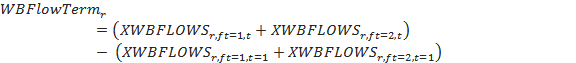
Finally, there are adjustments to reflect the possible impact of financial flows from international financial institutions (IFIs) such as the World Bank or International Monetary Fund (called XWBFLOWS independent of the source) and from foreign aid (AID). The IFI term represents the absolute difference between those flows in the current and initial years. The targets of those IFI flows are set exogenously via a parameter ( xwbsectar ) that is dimensioned by target of flow (ft), namely education, health, unskilled households, skilled households, and other. Funds for the first two targets go to government consumption and funds for the household targets go to transfer payments. Extensive documentation of the stocks and flows associated with IFI funds and the user control of them is provided elsewhere. The aid flow term takes into account the difference between current and initial net receipts, allocating a portion of this to government consumption (the rest will go to household transfers). The government consumption portion is proportional to the share of government consumption in the sum of government consumption and household transfers.

As an alternative to the structure described above, the project has experimented with the computation of GOVCON not from a single function, but as the sum of estimates of its various destination components such as military and education (the GDS vector discussed below), with each of those estimates computed as a function of GDP per capita). That is rather more complex than necessary; and the model’s currently quite rapid drop of infrastructure spending as a portion of GDP in the transition of low-income countries to middle-income ones tends to bring down or hold down the ratio of GOVCON to GDP more than historical data suggest occurs with development.

The division of government expenditures into target destination categories (GDS), part of the broader socio-political module of IFs is described later. That division is, of course, also a key agent-class behavior. With respect to sector of origin for government consumption (GS), which is information needed for the equilibration mechanism in the core commodities module, IFs simplistically assumes in the pre-processor (because of an absence of data or even qualitative information) that all government spending except arms, which has its source in manufactures, comes from services. On a year-to-year basis, the sectors of origin remained fixed at the initial proportions.

Government to Household Transfers  

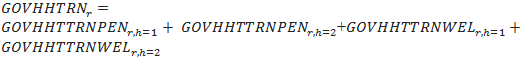
Government transfers, as distinguished from direct consumption expenditures, are computed using two different behavioral logics, a top-down one like the one for government consumption, and a bottom-up logic. The bottom-up logic is especially important in the analysis of pensions, because it is responsive to the changing size of the elderly population.

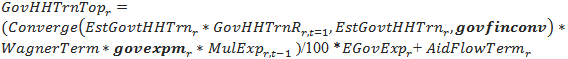
The top-down logic again uses an aggregate function responsive to changes in GDP per capita to calculate an estimated value of transfers as a portion of total government expenditures (EstGovtHHTrn).

The estimated value for the portion of total expenditures that household transfers constitute, adjusted by an initial shift term to accommodate initial data (GovHHTrnR), converges over time to the estimated value without the shift term. As with government consumption there is a Wagner term to represent possible growth with time, an exogenous multiplier for scenario analysis ( govexpm ) and an endogenously computed multiplier term to adjust government revenues and expenditures to each other (MulExp). That adjusted value is multiplied by an expected value for total government expenditures based on that in the preceding year, because the current value is not yet available.

where

Finally, there are adjustments to reflect the possible impact of financial flows from foreign aid (AID). The aid flow term takes into account the difference between current and initial net receipts, allocating a portion of this to government consumption (the rest goes to household transfers. The government transfer portion is proportional to the share of household transfers in the sum of government consumption and household transfers.

The bottom-up logic involves computing two terms, one for pensions and one for soi8cal welfare, in preparation for summing them. The pension term, like the top-down logic, also computes an initial estimate of pension expenditures (GovtPensions) as a portion of GDP using a function estimated cross-sectionally with GDP per capita at PPP. Not shown is an algorithm that ramps up that portion from 2 percent to 8 percent as GDP per capita at PPP climes from 0 to $8,000, over-riding the bottom portion of the analytical function below.

An initial estimate of government spending on pensions (GovtPensions) is calculated by multiplying this estimate, adjusted for the shift between estimate and actual value in the first year, by an adjustment portion by a potential relative price adjusted GDP (GDPPOTRPA).

where

Consistent with the bottom-up logic, that initial calculation is compared with a calculation that is built up from an estimate of the financial needs/demands of retired population. That second estimate looks at the size of the retired population, and multiplies that by per capita pension benefits in the first year, adjusted for the increase in GDP per capita. Given changing and often decreasing retirement ages, the retired population is a sum of those over age 65 and a term called RetirementPopAdj, which is computed to take into account an exogenous retirement age ( labretagem ). The larger of the analytically determined initial estimate and the retirement-population based numbers indicates the total pressure in the system for public pensions.

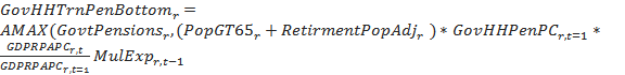
where

A further algorithmic check is made of the above calculation to limit per-person pension requirements as the size of the retired population grows from below 20 percent of the total population (in which case the limit is the average per capita GDP) to 40 percent or more of the total (in which case the limit is 70 percent of the average per capita GDP).

The bottom-up calculation of welfare transfers is parallel to that for pensions.

The total bottom-up transfer calculation is the sum of that for pension and welfare transfers.

The larger of the two numbers indicates the total pressure in the system for transfers to households.

Given these total transfers, there are further steps required to finalize the division into pension and welfare transfers and to divide each of those into transfers to skilled and unskilled households. The first step is an interim division of the total into pension and welfare categories using the bottom-up calculations.

The split to unskilled and skilled households is proportional to the share of their respective income in total household income and can be further affected by exogenous transfer parameters. The pension amounts are further adjusted by a pension multiplier (MulPen) that reflects the ratio of retirement needs (HHRETIRENEED) to life cycle consumption of those who are retired (CRETIRE) and helps equilibrate those two. The welfare amounts are further adjusted if net flows from international financial institutions (XWBFLOWS) have changed from initial conditions; those are added to the welfare transfers; welfare transfers are bounded to be below 20 percent of GDP.

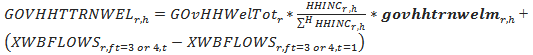
where

Finally, total government to household transfers are recalculated as the sum of the pension and welfare transfers to the unskilled and skilled households.