There a number of possible social, economic, and environmental impacts of infrastructure. We divided these into impacts on economic growth, income distribution, health, education, governance, and the environment. Given the limited empirical support for many of these linkages and, thus, a high level of uncertainty about whether and how to represent them, we have limited our inclusion of direct links from infrastructure to the links from infrastructure to economic growth and health. Important indirect linkages supplement the direct linkages that we describe here. For example, the forward linkages from economic growth to environmental impact (via paths such as increased energy use and food demand) and from improved health to demographic change are present in the current model. In fact, the indirect linkages via both of these paths are pervasive across the model.

Impacts on productivity and economic growth

We estimate the impact of infrastructure on economic growth through its effect on multifactor productivity. Most economic models relate aggregate growth to changes in factors of production, typically capital (K) and labor (L), and an additional component, which is variously called the Solow residual, the technological change parameter, total factor productivity (TFP) or multifactor productivity (MFP); here we use the MFP label. Analyses have long shown that MFP can be quite large (Solow 1956; 1957). Within IFs, we treat MFP as an endogenous variable that human capital, social capital, physical capital, and knowledge capital influence (Hughes 2007). Infrastructure is a key component of physical capital, along with natural resources. The impact of the latter is represented through the effect of energy prices on MFP.

In estimating the impact of infrastructure on MFP, we relate the impact to measures of physical infrastructure and not to measures of infrastructure spending. Because of the interaction effects across infrastructure types, we do not attempt to estimate the impact of individual forms of infrastructure but rather estimate the impact as a function of a composite index of infrastructure. Due to the very different historical and expected growth patterns of more traditional infrastructure—transportation, energy and water—vis-à-vis ICT, we create a separate index for ICT and link it to the physical capital component of MFP (MFPPC) in a different way.

Traditional Infrastructure – Transportation, Electricity, and Water and Sanitation

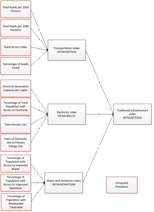
For the more traditional forms of infrastructure—transportation, electricity, and water and sanitation, we first construct a set of component indices—INFRAINDTRAN, INFRAINDELEC, and INFRAINDWATSAN (see the figure below). These are then aggregated into an overall index, INFRAINDTRAD.

In order to construct these indices, we followed the approach presented in Calderón and Servén (2010a). This begins with basic measures of infrastructure, e.g., the number of telephone lines, the amount of electricity generating capacity, and the length of the road network. These measures are ‘standardized’, as follows:

1. If the indicator is not already normalized by a meaningful scaling factor, e.g., land area or total population, calculate an appropriate normalized value. This is based on the notion that, for example, it makes more sense to compare countries based on the number of telephones per person rather than the total number of telephones. The following figure shows the normalized indicators used for each of the component indices.
2. The logarithms of the normalized indicators are calculated.
3. The mean and standard deviation for each of the normalized and logged indicators in the year 2010 are calculated in the pre-processor. These are stored in the vectors INFRAINDTRANCOMPMEANI, INFRAINDTRANCOMPSDI, INFRAINDELECCOMPMEANI, INFRAINDELECCOMPSDI, INFRAINDWATSANCOMPMEANI, and INFRAINDWATSANCOMPSDI, each of which has an entry for each indicator included in the component index.
4. In each forecast year, a z-value for each of the normalized indicators is calculated by subtracting the mean value for the year 2010 and then dividing by the standard deviation for the year. This provides a more standardized measure of the difference across countries and is independent of the original units of measure. If a country has negative (positive) z-value for a particular indicator, this indicates that its level of that indicator is smaller (greater) than it was for the average country in 2010. By definition, the aggregated z-value for the world for each indicator in 2010 is equal to 0.

The component indices are then calculated as a weighted sum of the z-values for the normalized indicators used for each of the component indices. The weights are given by the parameters infraindtrancompwt , infraindeleccompwt , and infraindwatsancompwt , where, once again each of these is a vector with an entry for each indicator included in the component index. Finally, the overall traditional infrastructure index, INFRAINDTRAD, is calculated as a weighted sum of the component indices. The weights are given by the parameter infraindtradcompwt , which is a vector with three entries, one for each of the component indices.

As with the z-values for the individual indicators, a negative (positive) value of for one the component indices or the overall index implies that a country ranks below (above) the average country in 2010 for that indicator. Furthermore, by definition, the aggregated value for the world for each index in 2010 is equal to 0.

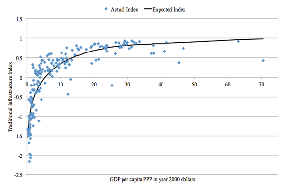
We use the overall Traditional Infrastructure Index to calculate the impact of traditional infrastructure on MFP in the same way as we do for most factors that influence MFP. As described by Hughes (2007: 15–16), we do this by comparing the value of INFRAINDTRAD to the value of INFRAINDTRADEXP, which is calculated using a benchmark function ^[1]  that indicates what value we would expect to see for a country given its current level of GDP per capita (see the figure below). A country whose index falls above (below) the benchmark value receives a boost to (reduction from) its MFP. For example, Gabon and Latvia have similar levels of GDP per capita in 2010, but Latvia’s Traditional Infrastructure Index falls well above the benchmark line, while Gabon’s falls well below. Thus, the former will receive a boost to its MFP due to traditional infrastructure, while the latter will receive a reduction.

The size of the boost or reduction depends on the distance from the benchmark value, INFRAINDTRAD – INFRAINDTRADEXP, and a factor relating this distance to productivity, which is given by the parameter mfpinfrindtrad . Calderón and Servén (2010a: i35) presented a value of 2.193 as their estimate of the increase in annual average growth rate of GDP per capita for an increase in 1 unit of their index. Based on this, we use a default value of 2 for the effect of traditional infrastructure on MFP. Specifically, if the value of the Traditional Infrastructure Index for a country is a full point above its expected value in a given year, it would receive a 2 percentage point boost to its MFP, which roughly translates into the same increase in growth in GDP per capita, over the coming year. The model user can change this value, allowing for exploration of the sensitivity of model results to the traditional infrastructure parameter.

ICT

The ICT Index, INFRAINDICT ^[2] , is calculated as a weighted average of the subscription rates for three of the four different kinds of ICT – mobile phones, fixed broadband, and mobile broadband. Since the subscription rates for mobile phones and mobile broadband saturate at 150 per 100 persons, their values are first multiplied by 2/3 so that they range from 0 to 100. The weights are given by the parameter infraindictcompwt , which is a vector with three entries, one for each of the component indices. By default, these values are set to 1, indicating equal weighting.

When considering the impact of ICT infrastructure on MFP, using the same approach as for traditional infrastructure would be problematic. Our formulation for forecasting ICT infrastructure includes a technology shift factor. Therefore, any relationship between GDP per capita and the expected level of ICT would not remain stable over time; for example, a country with a GDP per capita of $5,000 in 2015 would be expected to have more ICT infrastructure than a country with a GDP per capita of $5,000 in 2010.

We therefore associate the growth contribution from ICT advances with annual changes in the ICT Index, rather than with the level of the index as we do for traditional infrastructure. We multiply the annual unit change in the ICT Index by the parameter mfpinfrindict . Qiang, Rossotto and Kimura (2009: 45) estimated that each 10 percent increase in broadband penetration in developing countries increased the growth rate of per capita GDP by 1.38 percentage points (by 1.21 percentage points for developed countries) during the 1980 to 2006 period. We arbitrarily reduced the impact by using a default value of 0.8 because our index is a mixture of several types of ICT infrastructures, not all of which might have as strong an impact on economic productivity as does broadband. Thus, a 10 point increase in the value of the ICT index would result in a 0.8 addition to MFP, or an approximate increase of 0.8 percent in GDP per capita.

There is one obviously questionable implication of this approach. When a country reaches saturation in the ICT Index, it will no longer receive a productivity boost from ICT. Given the current rapid increase in mobile telephones and mobile broadband that together make up two-thirds of the ICT Index, we see in most scenarios a near-term boost to MFP from ICT in much of the world, followed by little or no contribution later in the horizon. Our uncertainty with respect to appropriate treatment of the longer-term contribution of ICT points to one of the limitations of trying to forecast rapidly changing technologies.

Impacts on health

There are many ways in which infrastructure can affect human health. We have chosen to limit our inclusion of these effects to a small set, specifically the impact of (1) unsafe water, sanitation, and hygiene directly on diarrheal diseases, and indirectly on diseases related to undernutrition; and (2) indoor air pollution on respiratory infections, such as pneumonia, and respiratory diseases, such as chronic obstructive pulmonary disease. These health outcomes are influenced directly by infrastructure via our measures of access to improved sources of drinking water and sanitation and the use of solid fuels in the home. These measures serve as proxies for the environmental health risks linked to infrastructure in IFs. We explored these effects in a previous volume in this series, Improving Global Health (B.Hughes, Kuhn, et al. 2011: 95–100), and have some confidence in the reasonableness of our results.

Our approach for estimating the impact of these health risks is described in the health documentation. Therefore, we provide only a brief overview here. In general, we compare the forecasted values of these infrastructure indicators to values that we would anticipate based only on income and educational attainment (distal drivers). If the estimated and expected values differ, we adjust the levels of mortality and morbidity for the associated diseases forecasted based only on the distal drivers. For example, if the levels of access to improved sources of water and sanitation are higher than expected, we reduce the mortality rate from diarrheal diseases. The amount by which the mortality rate is reduced is based on the analysis presented in the Comparative Risk Analysis work of the World Health Organization (Ezzati et al. 2004). This general approach, comparing forecasted values with expected ones and translating the difference into impact in a forward linkage, is fundamentally similar to the method described above for linking infrastructure development and economic productivity.

[1] This benchmark function is actually the combination of two functions: 1) INFRAINDTRADEXP = -0.881 + 0.519 * GDPPCPPP at levels of GDPPCPPP below $5000 and 2) INFRAINDTRADEXP = 2.767 + 0.225 * GDPPCPPP at levels of GDPPCPPP above $40000, with blending between these two thresholds.

[2] A separate index, INFRAINDICTZ , is also calculated following the same approach as for the component indices of traditional infrastructure. This is only used for display purposes.