Conceptual foundations of distribution in IFs: The Lorenz Curve and Gini Coefficient

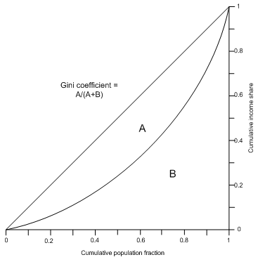
The Lorenz curve is the most widely used method for representing inequality in earnings, income, or wealth (see the figure below). It portrays the cumulative share of income (or any other quantity distributed across a population) held by increasingly well-to-do cumulative shares of population. The more equally distributed a factor is, the closer the Lorenz curve will be to the hypotenuse of the right-triangle, sometimes called the line of equality. The Gini coefficient is the “area of inequality” immediately below the hypotenuse (A) divided by the area of the triangle (A+B); thus larger Gini coefficients indicate greater inequality. 

The Lorenz curve is “non-parametric” in the sense that it is an empirical distribution that is an accurate representation of survey data on income or consumption for a society. While the Lorenz curve is useful conceptually, to capture the dynamically evolving distribution of income or consumption it is more convenient to have an analytic or “parametric” representation of the distribution. Moreover, we would like a representation from which we can conveniently compute specific deciles or quintiles (thereby reconstructing the Lorenz curve) and also compute key poverty measures like the headcount. The most widely used parametric representation is the lognormal density. We will not describe that function here. Because we relate the Gini coefficient to a lognormal function in our forecasting of poverty rates, please see the documentation of poverty forecasting for that discussion. Here we will focus only on the forecasting of the Lorenz curve in IFs and the calculation of the Gini coefficient from that forecasting.

The challenge for IFs forecasting of distribution becomes the forecasting of the Lorenz curve itself; calculation of Gini is simple once we have that curve at any time point for any population. Forecasting the Lorenz curve necessarily involves the forecasting of the differential performance of segments within the population. Based on historic data, the income means of different deciles could be extrapolated or in some other way forecast, but such extrapolation would be unrelated to the rest of the IFs model (including specific interventions that might change those means) and would add nothing much simply to extrapolating changes in Gini itself.

Ideally, the forecasting of segments of population from poorest to richest across the Lorenz curve should be tied to an elaboration of household types as is done with a Social Accounting Matrix (SAMs). SAMs can distinguish multiple types of urban and rural households and their changing demographic sizes (as a result, for instance, of rural-to-urban migration) and income structures (as a result of structural change in the economy, of changing patterns of government transfers, and many other factors). For the purposes of studying longer-term change in global poverty levels in IFs the SAM ideal is tarnished by two realities: (1) in spite of efforts via the UN’s System of National Accounts, there is no standard household classification system for SAMs; they vary widely and are generally used in single-country analysis, not global forecasting; and (2) most models built around SAMs are used for rather short-term analysis and even more commonly for comparative static analysis (for example, comparison of income patterns in a society not open to agricultural imports to one that is, without much or any consideration of the dynamic path from one to the other).

Nonetheless, the basic rooting of forecasts of a Lorenz curve and therefore of Gini in a SAM retains the tremendous advantage of tying those forecasts to changes in clearly policy-relevant interventions. And fortunately, the Global Trade and Analysis Project (GTAP) has collected key information, such as share taken of value added, about two classes of households, those based respectively on skilled and unskilled labor, across the large number of countries/ regions and economic sectors that the project covers (see https://www.gtap.agecon.purdue.edu/default.asp). IFs has drawn heavily on the GTAP data, updating regularly to the most recent version, in its own economic model structure and built the IFs SAM on the basis of the two household categories. The GTAP database has made it possible to develop forecasts of income by type of household as economies and therefore value added shares shift from agriculture to manufacturing and to services. (See the documentation topic on Household and Firm Income.)

Although it is far from ideal to have only two categories of population (unskilled and skilled), it is possible to represent a Lorenz Curve showing what portion of income the unskilled (poorer) portion of the population obtains, specifying one point on the Lorenz curve that will fall below the diagonal (the line of equality). The unskilled and skilled portions together will receive all of the income. Although simple this Lorenz curve (actually two line segments), allows calculation of Gini.

For the purposes of forecasting, we need only forecast two things: the changing shares of income of the two groups and the changing sizes of the two groups. The GTAP database facilitates the forecasting of income shares because it indicates income patterns for the two population groupings by economic sector and, across all of the countries in GTAP, helps us abstract changing patterns of those sector shares with change in GDP per capita at PPP. The documentation of household income by household type describes how that is done in IFs.

This leaves one further challenge for forecasting, the determination of the split of the population between unskilled and skilled households. Unfortunately, the GTAP dataset does not provide numbers on labor force size, only on sector income shares. And OECD data on labor force size by classification such as professional and administrative, which could be used to estimate numbers of skilled versus unskilled workers, exist only for well-to-do countries. Moreover, we need not only initial conditions, but forecasting formulations. Although we would expect that the portion of the population that is skilled would grow with the educational level of the population, the relationship is complex, in part because (1) more advanced economies may set a higher bar for determining what a skilled worker is and (2) more highly educated populations may find that there is credential inflation that effectively demotes some with education to a less skilled category.

Therefore formulations and algorithms for both the initialization and forecasting of skilled and unskilled numbers are necessary. IFs has used two different processes to help generate rough estimates of the numbers, a legacy procedure that we document because some variation of it may still have value in the future, and a second, currently used process. 

An earlier, legacy process to compute domestic Gini

The earlier process involved looking at the formal educational attainment levels of the adult population. The cross-sectional graph below shows the portion of the population 25 years and older with tertiary education plus ½ of that with secondary education. That is a very arbitrary and crude definition of skilled labor, but is a starting point. The value of tying the size of skilled and unskilled labor forces to education completion is that the education module of IFs forecasts sizes of population with various educational attainment levels and those can be driven by agent-class interventions. And it is the change in share of skilled labor that is most important, not the absolute numbers—the Gini coefficient data can be used to adjust the initial conditions of income distribution and the change in labor force sizes can help us forecast the change in Gini.

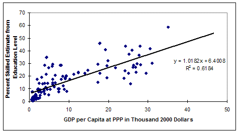
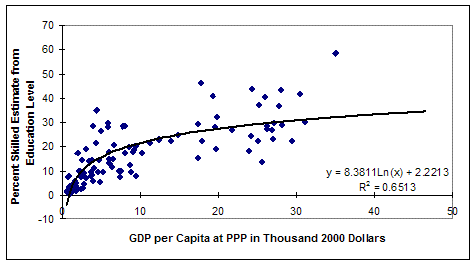
There are some obvious problems with the graph above. One of the most significant is that better fits are achieved by other functional forms, including the logarithmic one below. Unfortunately, those forms tend to suggest that the poorest countries have absolutely no skilled labor, clearly an exaggeration.

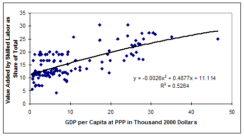
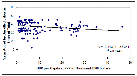
How do we know that an absence of skilled labor in the poorest countries is an exaggeration? In addition to common sense, it can be seen from the GTAP data on the income share of skilled labor in the graph below. That shows that they obtain a substantial share of value added even at the lowest levels of GDP per capita. The two cross-sectional graphs below show the shares of value added accruing to skilled and unskilled labor, respectively.

The current process in IFs to compute domestic and global Gini coefficients

An earlier procedure for computing Gini linking skilled labor to those with a tertiary education and half of those with a secondary education was formerly used in IFs. But it had some instability and unanticipated consequences, in part because the reality is there is credential inflation; as countries become richer, fewer and fewer of those with tertiary education, much less secondary, are considered adequately skill. Therefore the model has been switched to one that looks at the average years of education held by adults 15 years of age and over (EDYRSAG15).

The process begins by using a function estimated from the relationship between GDPPCP and GTAP data on the share of value added accruing to skilled workers to estimate the share of the labor force that is skilled (PerSkilled); that will be wrong, but remember that we do not need the exact share, what we need is the change over time. And the model uses that same function over time to estimate the expected share of skilled labor, all else equal, over time. But all is not equal and it is unequal to the extent that education levels rise higher than those that we would expect in the same development process. Hence there is an adjustment term in the calculation (LabSupSkillAdj) that looks at the difference between the actual years of education in the population and the expected years (YearsEdExp), again computed by an analytical function with GDP per capita at PPP. A fraction of the proportional difference of actual with expected is added to the percentage skilled.

where

Given the percentage skilled it is simple to calculate the number skilled (LABSUP) and the residual percentage of the labor force that is unskilled.

Levels of skill in the labor force are used to estimate household populations with associated skills (recognizing that household sizes in different skill categories may actually be unequal).

Given the income shares accruing to skilled and unskilled shares of the population and the sizes of those portions of the population, the domestic Gini index (GINIDOM) is computed from the simple Lorenz curve that those two incomes and population shares create, scaled to the empirically known initial condition. The calculation in the Lorenz curve function GinDomCalcFunc is modified by a scaling or shift parameter (GINIDomRI) so that the initial condition is preserved. A multiplier parameter ( ginidomm ) can change the calculation over time.

where

There is, however, an alternative and completely exogenous way of calculating Gini, if the parameter ginidomr has a value greater than 0. In that case, the value of Gini is simply the initial condition changed over time by ginidomr (again modified, if desired, by ginidomm ).

IFs also calculates two variations of a global Gini index to supplement the country-specific one. The first is a Gini coefficient (GINI) that describes the distribution of income across all countries, using country incomes as the unit of analysis. 

That measure does not take into account income distribution within countries. The second global Gini measure (GINIFULL) does take into account income distributions both within and across countries (subject, of course, to the limitation that IFs represents domestic income distribution only as a function of two income categories). That makes it essentially a measure of global income distribution at the individual human level, rather than the country level. 

Finally, the user interface of IFs uses the same Lorenz-curve approach to allow the user to calculate a specialized-display GINI for any variable that can be represented across all countries/regions of the model.