 International Futures at the Pardee Center
International Futures Help System
Equations: Student Flow
Econometric Models for Core Inflow and Outflow
Enrollments at various levels of education - EDPRIENRN, EPRIENRG, EDSECLOWENRG, EDSECUPPRENRG, EDTERENRG - are initialized with historical data for the beginning year of the model. Net change in enrollment at each time step is determined by inflows (intake or transition) and outflows (dropout or completion). Entrance to the school system (EDPRIINT, EDTERINT), transition from the lower level (EDSECLOWRTRAN, EDSECUPPRTRAN) - and outflows - completion (EDPRICR), dropout or it's reciprocal, survival (EDPRISUR) - are some of these rates that are forecast by the model.
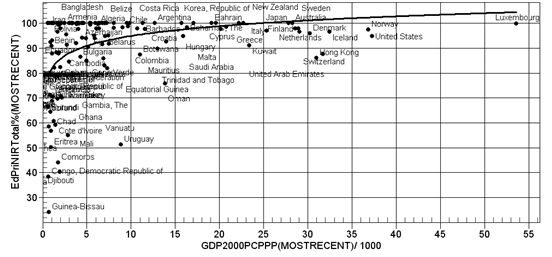
The educational flow rates are best explained by per capita income that serves as a proxy for the families' opportunity cost of sending children to school. For each of these rates, separate regression equations for boys and girls are estimated from historical data for the most recent year. These regression equations, which are updated with most recent data as the model is rebased with new data every five years, are usually logarithmic in form. The following figure shows such a regression plot for net intake rate in elementary against per capita income in PPP dollars.
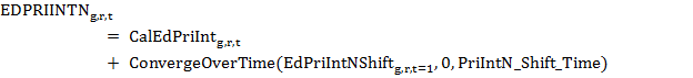
In each of the forecast years, values of the educational flow rates are first determined from these regression equations. Independent variables used in the regression equations are endogenous to the IFS model. For example, per capita income, GDPPCP, forecast by the IFs economic model drives many of the educational flow rates. The following equation shows the calculation of one such student flow rate (CalEdPriInt) from the log model of net primary intake rate shown in the earlier figure.
![]()
While all countries are expected to follow the regression curve in the long run, the residuals in the base year make it difficult to generate a smooth path with a continuous transition from historical data to regression estimation. We handle this by adjusting regression forecast for country differences using an algorithm that we call "shift factor" algorithm. In the first year of the model run we calculate a shift factor (EDPriIntNShift) as the difference (or ratio) between historical data on net primary intake rate (EDPRIINTN) and regression prediction for the first year for all countries. As the model runs in subsequent years, these shift factors (or initial ratios) converge to zero or one if it is a ratio (code routine ConvergeOverTime in the equation below) making the country forecast merge with the global function gradually. The period of convergence for the shift factor (PriIntN_Shift_Time) is determined through trial and error in each case.
The base forecast on flow rates resulting from of this regression model with country shift is used to calculate the demand for funds. These base flow rates might change as a result of budget impact based on the availability or shortage of education budget explained in the budget flow section.
Systemic Shift
Access and participation in education increases with socio-economic developments that bring changes to people's perception about the value of education. This upward shifts are clearly visible in cross-sectional regression done over two adequately apart points in time. The next figure illustrates such shift by plotting net intake rate for boys at the elementary level against GDP per capita (PPP dollars) for two points in time, 1992 and 2000.
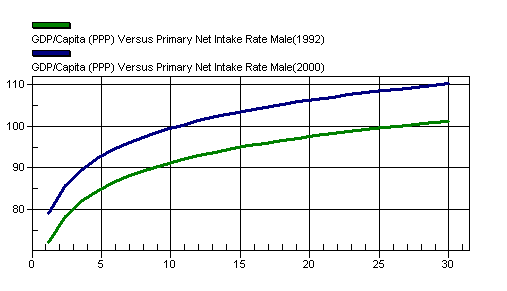
IFs education model introduces an algorithm to represent this shift in the regression functions. This "systemic shift" algorithm starts with two regression functions about 10 to 15 years apart. An additive factor to the flow rate is estimated each year by calculating the flow rate (CalEdPriInt1 and CalEdPriInt2 in the equations below) progress required to shift from one function, e.g., to the other, s, in a certain number of years (SS_Denom), as shown below. This systemic shift factor (CalEdPriIntFac) is then added to the flow rate (EDPRIINTN in this case) for a particular year (t) calculated from regression and country shift as described in the previous section.
![]()
![]()
![]()
![]()
As said earlier, Student flow rates are expressed as a percentage of underlying stocks like the number of school age children or number of pupils at a certain grade level. The flow-rate dynamics work in conjunction with population dynamics (modeled inside IFs population module) to forecast enrollment totals.
Grade Flow Algorithm
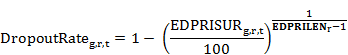
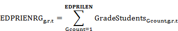
Once the core inflow (intake or transition) and outflow (survival or completion) are determined, enrollment is calculated from grade-flows. Our grade-by-grade student flow model therefore uses some simplifying assumptions in its calculations and forecasts. We combine the effects of grade-specific dropout, repetition and reentry into an average cohort-specific grade-to-grade dropout rate, calculated from the survival rate (EDPRISUR for primary) of the entering cohort over the entire duration of the level (EDPRILEN for primary). Each year the number of new entrants is determined by the forecasts of the intake rate (EDPRIINT) and the entrance age population. In successive years, these entrants are moved to the next higher grades, one grade each year, subtracting the grade-to-grade dropout rate (DropoutRate). The simulated grade-wise enrollments (GradeStudents with Gcount as a subscript for grade level) are then used to determine the total enrollment at the particular level of education (EDPRIENRG for Primary).
There are some obvious limitations of this simplified approach. While our model effectively includes repeaters, we represent them implicitly (by including them in our grade progression) rather than representing them explicitly as a separate category. Moreover, by setting first grade enrollments to school entrants, we exclude repeating students from the first grade total. On the other hand, the assumption of the same grade-to-grade flow rate across all grades might somewhat over-state enrollment in a typical low-education country, where first grade drop-out rates are typically higher than the drop-out rates in subsequent grades. Since our objective is to forecast enrollment, attainment and associated costs by level rather than by grade, however, we do not lose much information by accounting for the approximate number of school places occupied by the cohorts as they proceed and focusing on accurate representation of total enrollment.
![]()
![]()
Gross and Net
Countries with a low rate of schooling, especially those that are catching up, usually have a large number of over-age students. Enrollment and entrance rates that count students of all ages are called gross rates in contrast to the net rate that only takes the of-age students in the numerator of the rate calculation expression. UNESCO report net and gross rates separately for entrance and participation in elementary. IFs education model forecasts both net and gross rate in primary education. An overage pool (PoolPrimary) is estimated at the model base year using net and gross intake rate data. Of-age non-entrants continue to add to the pool (PoolInflow). The pool is exhausted using a rate (PcntBack) determined by the gross and net intake rate differential at the base year. The over-age entrants (cOverAgeIntk_Pri) gleaned from the pool are added to the net intake rate (EDPRIINTN) to calculate the gross intake rate (EDPRIINT).
![]()
![]()
![]()
![]()
![]()
![]()
Vocational Education
IFs education model forecasts vocational education at lower and upper secondary levels. The variables of interest are vocational shares of total enrollment in lower secondary (EDSECLOWRVOC) and the same in upper secondary (EDSECUPPRVOC). Country specific vocational participation data collected from UNESCO Institute for Statistics do not show any common trend in provision or attainment of vocational education across the world. International Futures model initialize vocational shares with UNESCO data, assumes the shares to be zero when no data is available and projects the shares to be constant over the entire forecasting horizon.
IFs also provides two scenario intervention parameters for lower (edseclowrvocadd) and upper secondary (edsecupprvocadd) vocational shares. These parameters are additive with a model base case value of zero. They can be set to negative or positive values to raise or lower the percentage share of vocational in total enrollment. Changed vocational shares are bound to an upper limit of seventy percent. This upper bound is deduced from the upper secondary vocational share in Germany, which at about 67% is the largest among all vocational shares for which we have data. Changes to the vocational share through the additive parameters will also result in changes in the total enrollment, e.g., EDSECLOWRTOT for lower secondary, which is calculated using general (non-vocational) enrollment (EdSecTot_Gen) and vocational share, as shown in the equations below (for lower secondary).
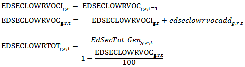
Forecasts of EdSecTot_Geng,r,t is obtained in the full lower secondary model using transition rates from primary to lower secondary and survival rates of lower secondary.
Science and Engineering Graduates in Tertiary
Strength of STEM (Science, Technology, Engineering and Mathematics) programs is an important indicator of a country’s technological innovation capacities. IFs education model forecasts the share of science and engineering degrees (EDTERGRSCIEN) among all tertiary graduates in a country. Data for this variable is available through UNESCO Institute for Statistics. The forecast is based on a regression of science and engineering share on average per person income in constant international dollar (GDPPCP). There is an additive parameter (edterscienshradd), with a base case value of zero, that can be used to add to (or subtract from) the percentage share of science and engineering among tertiary graduates. This parameter does not have any effect on the total number of tertiary graduates (EDTERGRADS).
![]()