Given its advantages, the IFs approach to forecasting poverty uses the lognormal formulation, driven by average income (actually household consumption) and the Gini coefficient. One advantage of the approach is that the two drivers (average consumption and the log-normal function/distribution linked to Gini) allow the computation of poverty rates at any poverty level specified and a specialized poverty display within the IFs system allows the user to do just that. Yet to be consistent with the Millennium Development Goals and the common discourse we focus on levels such as $1.25 and $2.00 per day, specified in terms of purchasing power. The computed variables in IFs use those levels (INCOMELT1LN and INCOMELT2LN).

Although it is common to speak of poverty in terms of income, much of the survey data used to identify historical and contemporary levels has focused on consumption and the IFs calculations are driven by household consumption per capita (C divided by POP). Another and related important decision was the use of changes of household consumption to drive poverty over time—although survey data from the World Bank's PovcalNet database are used to initialize poverty rates and numbers, C and domestic income distribution (GINIDOM) change values over time. It is well-know that calculations from national accounts data tend to provide lower poverty rates than those found in surveys. IFs computes shift factors in the first year that identify the ratio of values from surveys to those from national accounts (NSNARAT) and maintains those shifts over time (although an exogenous parameter, nsnaratm can adjust those over time). Another exogenous parameter can change the poverty level from $1 ( incomepovlevm ).

The process in IFs begins with the calculation of the lognormal standard deviation (LNStDev) from Gini and with the calculation of the mean consumption (MeanConsumption) from consumption per capita and a smoothed conversion factor from market exchange rates to purchasing power parity (SmPPPConv). These are the key drivers of the lognormal formulation. See Appendix 2 of Hughes et al. (2009) for a more formal and extended explanation of the entire poverty calculation system using the lognormal approach.

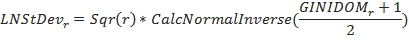
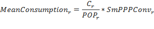
where

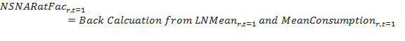
Given these driving inputs, IFs uses a two-step process for calculating the share of population below any given consumption level. The first step produces a log normal mean (LNMean) based on the mean consumption adjusted by the national accounts scaling factor from the first year (NSNARatFac) and the lognormal standard deviation.

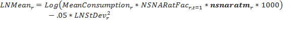
where

Finally, a specialized function computes the rate of poverty to be multiplied by the population to get the poverty numbers.

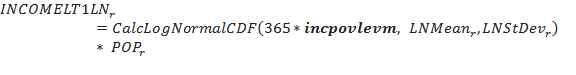
The calculation of poverty below $2 is the same, except that the value of 365 in the above equation becomes 365 * 2 = 730.

In 2014 the International Comparison Project (ICP) rebased its estimates for all countries of GDP at purchasing power from 2005 values and dollars (at PPP) to 2011 values and re-estimated PPP values. In order to pick up new estimates of income poverty, IFs added two new variables, one for poverty at $1.25 in 2011 PPP dollars (INCOMLET1LN2011) and another similarly for poverty at $0.70 (INCOMELT07LN2011). It was necessary to re-estimate the appropriate value of household consumption (C) for these estimates. In the sequence of calculations above this was possible with the reformulation below (and related changes for the $0.70 calculation):

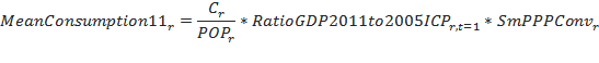
where

The calculation of the poverty gap at $1.25 (POVGAP) relies on the same basic lognormal structures and some of the same input variables. The poverty gap is defined as the mean shortfall from the poverty line, expressed as a percentage of the poverty line; the non-poor are considered to have zero shortfall. The measure helps identify the depth of poverty and is therefore a useful supplement to its incidence.

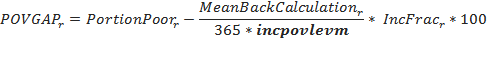
where