It is important to recognize not just the initial empirical (or estimated) value of smoking rate in our base year for each country, but the trajectory of country-specific change in smoking rates. Our approach to capturing the trajectory is a variation on a moving-average approach.  Every year our first step is to compute a compound growth rate of the smoking rate over the last 10 years.  In the second step we also compute the rate of change that one would expect based solely on applying the cross-sectional formulation in two consecutive years.  The third step is to compute a slowly-changing moving average by combining those two growth rate computations, weighting the compound historical growth rate 90 percent and the expectation of growth from the cross-sectional formulation 10 percent.

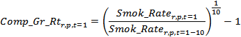
In the first step described above we obtain every year the compounded growth rate (Comp_Gr_Rt) over the previous 10 years. That growth rate is based on historical (or constructed) smoking rate data (Smok_Rate). ^[1]

In the second step described above we compute the annual expectation of growth in the smoking rate (Exp_Gr_Rt) based on the cross-sectional formulation expectations (Smok_Rate_Exp) for the current and previous year.

In the third step, every year we compute what is effectively a moving average of change in smoking rates (Mov_Gr_Rt) by combining the compound growth rate for the last 10 years with the expected value from the preceding to the current year (with 90 percent and 10 percent weighting, respectively). 

In the above computation we introduced a number of other algorithmic rules to produce what appeared to be reasonable forecasts of smoking rates given the general notion of a bell-shaped curve (or rise and then fall) of smoking with income and time. These included bounding the cross-sectional expected value formulations at $30,000 for females and $50,000 for males so as to avoid complete collapse of smoking rates at high income levels.

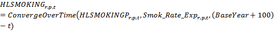
It is then possible to apply the moving average to obtain what is actually a preliminary forecast of smoking rate (although not used in the model, we can call it HLSMOKINGP) based on that in the previous year.

This preliminary smoking rate is then converged to match the result of the regression equation over a period of 100 years and yield a near final smoking rate (HLSMOKING)

High income countries (with initial GDP per capita at PPP or GDPPCPI > $25,000) then are checked to avoid smoking rate growth after they have started to drop, i.e:

If GDPPCPI > $25,000

and  >  

and  <=  

then  = 

Finally, a multiplier ( hlsmokingm ) by country and sex is available and applied to the smoking rate to compute the final value for the country-sex-year; the default value of the multiplier is 1 and alternative values introduce scenarios. Note that having a multiplier for a specific sex (e.g. 0.9 for males) and another for “total” or both sexes (e.g. 0.8) will produce a multiplicative effect on the forecast of 0.72.  This ability to stack multipliers for individual sexes with total or both is not the standard practice in IFs; this may be the only example of it.